Parallel Quantum Solutions

since 1997

• Home
• Machines
• Software
• Capabilities
• Benchmarks
• Pricing
• Documentation
• About
• Contact

News

04/23/12

PQSMol 2.0 revision 3 for Mac OS X is available now. Please visit the software section to download.

04/16/12

PQS 4.0 revision 4 is available now. It is a free upgrade for 4.0 users. Please visit the software section to download.

03/13/12

Intel Sandy Bridge 8-core based QuantumCubes^TM and AMD Interlagos 12- and 16-core based QuantmCubes^TM are available now. Please visit the machines section for details.

11/14/11

Website/email disruption. On Friday 11/11/11 our 10 year domain name registration expired. As a result we were unreachable via our website or email until Monday 11/14/11. We apologize for any inconvenience.

10/26/11

PQS 4.0 revision 3 is available now. It is a free upgrade for 4.0 users. Please visit the software section to download.

09/13/11

PQS 4.0 revision 2 is available now. It is a free upgrade for 4.0 users. Please visit the software section to download.

09/09/11

PQSMol 2.0 revision 1 is now available for Linux. It is a free upgrade for 2.0 users. The Trial version does not require a license and is free to download.

SUPPORT

by phone: (CST)
M-F 9:30am - 5:00pm
1-877-759-2777 or
1-479-521-5118.

by email:
general/customer service
sales@pqs-chem.com
technical support
tech@pqs-chem.com

Documentation

Manuals and Guides

• PQS Manual (PDF)
• PQSMol Manual (PDF)
• PQS installation instructions and overview (TXT)

Tutorials

• Tutorial 1 - Orbitals and Vibrational Frequencies in Lactic Acid
  • 1.1 Building the Lactic Acid molecule
  • 1.2 Creating a PQS input file
  • 1.3 Submitting the PQS job
  • 1.4 Visualizing the PQS job output
• Tutorial 2 - VCD spectrum of CHFClBr
  • 2.1 Building CHFClBr
  • 2.2 Creating a PQS input file
  • 2.3 Submitting a PQS job
  • 2.4 Visualizing the PQS job output
• Tutorial 3 - Methoxy Substitution in Perfluoroanthracene
  • 3.1 Building Perfluoroanthracene
  • 3.2 Creating a PQS input file
  • 3.3 Submitting a PQS job
  • 3.4 Visualizing the PQS job output
  • 3.5 Building 1-Methoxy-Perfluoroanthracene
  • 3.6 Visualizing the PQS job output
  • 3.7 Building 2- and 9-Methoxy-Perfluoroanthracene and Visualizing the PQS job outputs
  • 3.8 Comparing the NMR Spectra of perfluoroanthracene, 1-, 2-, and 9-methoxy- perfluoroanthracene

Tutorial 1.4 Visualizing the PQS job output

Step 11
Visualize the output.

As soon as the job finishes PQSMOL is launched in View mode in a separate window with the current job output file as an argument producing the window in Figure .

View window - initial display

Step 12
Examine the calculated molecular orbitals.

Press the Orbitals button the toolbar at the bottom of the View window
. Select the HOMO (#24) in the list on the right side of the window. A line representing the energy level of the 24$^{th}$ orbital is highlighted in red, see Figure .

Orbitals window - HOMO selected

The corresponding view window, displaying the HOMO is shown in Figure . Move the Isosurface level slider to change the isosurface displayed in the View window. Also, experiment with the Cross Sections sliders to produce various display results.

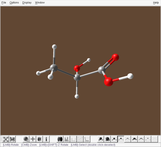
View window - HOMO displayed

Select other molecular orbitals in the list to see their display in the View window. Try changing the default settings in the Display→View window, including changing the grid resolution under Display→Orbital→Grid Resolution.

Step 13
Save a screen shot from the View window.

Once you have produced a "publication-quality" image in the View window, you can save it in JPEG format via the popup menu. Right-click anywhere within the View window and select the Capture menu item. A dialog prompting for a filename appears, Figure .

Save Image dialog

You may save the image under the suggested name mol_capture1.jpg in the current working directory by simply pressing the OK button. To turn off the MO display either toggle the state of the Orbitals button in the toolbar or close the Orbitals window.

Step 14
Examine the Vibrational spectrum.

To display the simulated IR spectrum click on the Vibrational Frequencies button in the toolbar at the bottom of the View window. The simulated IR spectrum is shown in Figure .

Vibrational Frequencies window - IR spectrum, mode #1 selected

The list on the right side of the Vibrational Frequencies window allows access to all of the vibrational frequencies of the molecule (30 in this example). Select the first frequency. A small red arrow appears under the corresponding frequency in the vibrational spectrum and details for that mode appear in green font at the top of the window (mode number, symmetry, frequency and intensity). This mode is primarily a twisting about the C-O bond and has a low intensity that does not show up in the simulated IR spectrum.

Now, activate the Vectors checkbox in the bottom left corner of the window, as shown in Figure . This will show the atomic displacements in the vibrational mode #1 as yellow vectors at each atom of the structure in the View window, Figure . Activate the Animate checkbox to animate the structure by showing the motion in the vibrational mode #1.

View window - vibrational mode #1 displacement vectors

Other vibrational modes can be selected from the list at the right side of the Vibrational Frequencies window or by directly selecting the peak in the simulated spectrum.

Vibrational Frequencies window - IR spectrum, mode #24 selected

View window - highest intensity vibrational mode #24 displacement vectors

Figure shows the displacement in the most intense IR mode #24 and Figure shows the corresponding Vibrational Frequencies window, with the peak highlighted in red.

[PREV]

Copyright © 2011 Parallel Quantum Solutions; All right reserved.